1
2
3
4
5
6
7
8
9
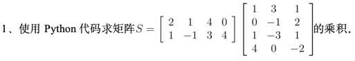
| import numpy as np
A = np.array([[2, 1, 4, 0],
[1, -1, 3, 4]])
B = np.array([[1, 3, 1],
[0, -1, 2],
[1, -3, 1],
[4, 0, -2]])
S = np.dot(A, B)
print(S)
|
[[ 6 -7  8]
 [20 -5 -6]]
2、编程解决如下投入产出问题:某县区有A、B、C三个企业,A企业每生产l元的产品要消耗0.4元B企业的产品和0.3元C企业的产品;B企业每生产l元的产品要消耗0.7元A企业的产品、0.l2元自产的产品和0.2元C企业的产品;C企业每生产l元的产品要消耗0.6元A企业的产品和0.l5元B企业的产品。如果这3个企业接到的外来订单分别为7万元、8.5万元和5万元,那么他们各生产多少才能满足需求?模型假设:假设不考虑价格变动等其他因素。
1
2
3
4
5
6
7
8
9
10
11
12
13
14
15
16
17
18
19
20
21
22
23
| import numpy as np
A = np.array([
[0, 0.7, 0.6],
[0.4, 0.12, 0],
[0.3, 0.15, 0]
])
d = np.array([70, 85, 50])
I = np.identity(3)
x = np.linalg.solve(I - A, d)
print("A企业需要生产的产品总额(万元):", x[0])
print("B企业需要生产的产品总额(万元):", x[1])
print("C企业需要生产的产品总额(万元):", x[2])
|
A企业需要生产的产品总额(万元): 382.5197238658777
B企业需要生产的产品总额(万元): 270.46351084812625
C企业需要生产的产品总额(万元): 205.32544378698225
3、编程解决如下问题:—个家禽养殖基地每天投入2元资金用于饲料、设备、人力,估计可使一只2千克重的鹅每天增加0.1千克。目前鹅出售市场价格为每千克30元,但是预测每天会降低0.04元。该基地应该什么时候出售这批鹅?如果上面的估计和预测有出入,那么对结果有多大影响?
1
2
3
4
5
6
7
8
9
10
11
12
13
14
15
16
17
18
19
20
21
22
23
| import numpy as np
from scipy.optimize import minimize_scalar
initial_weight = 2
weight_gain_per_day = 0.1
initial_price_per_kg = 30
price_decrease_per_day = 0.04
daily_investment = 2
def profit(days):
total_weight = initial_weight + days * weight_gain_per_day
price_per_kg = initial_price_per_kg - days * price_decrease_per_day
total_revenue = total_weight * price_per_kg
total_cost = days * daily_investment
return -(total_revenue - total_cost)
result = minimize_scalar(profit, bounds=(0, 500), method='bounded')
optimal_days = result.x
print(f"在第{round(optimal_days)}天出售")
|
在第115天出售
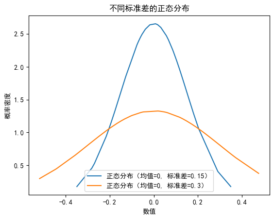
4、用Python编程实现如何获得两组模拟的正态分布的数据并输出结果。正态分布模拟的标准差为δ=0.l5和δ=0.3的两组数据,共40个点,通过matplotlib模块绘制出曲线图。
1
2
3
4
5
6
7
8
9
10
11
12
13
14
15
16
17
18
19
20
21
22
23
24
25
26
27
28
29
30
31
32
33
34
35
| import matplotlib.pyplot as plt
import numpy as np
from matplotlib.font_manager import FontProperties
plt.rcParams['font.sans-serif'] = ['SimHei']
plt.rcParams['axes.unicode_minus'] = False
mean_1, mean_2 = 0, 0
std_dev_1, std_dev_2 = 0.15, 0.3
n_points = 40
data_1 = np.random.normal(mean_1, std_dev_1, n_points)
data_2 = np.random.normal(mean_2, std_dev_2, n_points)
sorted_data_1 = np.sort(data_1)
sorted_data_2 = np.sort(data_2)
fit_1 = 1 / (std_dev_1 * np.sqrt(2 * np.pi)) * np.exp(-0.5 * ((sorted_data_1 - mean_1) / std_dev_1)**2)
fit_2 = 1 / (std_dev_2 * np.sqrt(2 * np.pi)) * np.exp(-0.5 * ((sorted_data_2 - mean_2) / std_dev_2)**2)
plt.plot(sorted_data_1, fit_1, label=f'正态分布(均值={mean_1}, 标准差={std_dev_1})')
plt.plot(sorted_data_2, fit_2, label=f'正态分布(均值={mean_2}, 标准差={std_dev_2})')
plt.legend()
plt.title('不同标准差的正态分布')
plt.xlabel('数值')
plt.ylabel('概率密度')
plt.show()
|
5、使用批量梯度下降算法拟合多维数据。待拟合的数据点为样本点对应的x值:[[6, 2], [8, 1], [10, 0], [14, 2], [18, 0]]),样本点对应的y值:[19, 21, 23, 43, 47])。上述数据点是根据函数y=3x1+4x2-7生成的。
1
2
3
4
5
6
7
8
9
10
11
12
13
14
15
16
17
18
19
20
| import numpy as np
def batch_gradient_descent(X, y, learning_rate=0.001, n_iterations=1000):
m, n = X.shape
X_b = np.c_[np.ones((m, 1)), X]
theta = np.zeros((n + 1, 1))
for iteration in range(n_iterations):
gradients = 2/m * X_b.T.dot(X_b.dot(theta) - y)
theta -= learning_rate * gradients
return theta
X = np.array([[6, 2], [8, 1], [10, 0], [14, 2], [18, 0]])
y = np.array([19, 21, 23, 43, 47]).reshape(-1, 1)
theta = batch_gradient_descent(X, y)
print(theta)
|
[[-0.36773111]
 [ 2.59937037]
 [ 2.27070972]]
6、某配送中心为所属的几个超市配送某品牌的厨具,假设超市每天对这种厨具的需求量是稳定的,订货费与每套产品每天的存贮费都是常数。如果超市对这种厨具的需求是可以缺货的,试编程制定最优的存贮策略。假设日需求为l00元,一次订货费为5000元,每套厨具每天的存贮费为l元,每套厨具每天的缺货费为0.l元。
1
2
3
4
5
6
7
8
9
10
11
12
13
14
15
16
17
18
19
20
21
22
| import numpy as np
def calculate_total_cost(demand_per_day, ordering_cost, holding_cost_per_unit, shortage_cost_per_unit, order_quantity):
days = order_quantity / demand_per_day
total_holding_cost = 0.5 * order_quantity * holding_cost_per_unit * days
total_shortage_cost = 0.5 * demand_per_day * shortage_cost_per_unit * days
total_ordering_cost = ordering_cost
return total_ordering_cost + total_holding_cost + total_shortage_cost
demand_per_day = 100
ordering_cost = 5000
holding_cost_per_unit = 1
shortage_cost_per_unit = 0.1
order_quantities = np.arange(demand_per_day, 5000, 100)
costs = [calculate_total_cost(demand_per_day, ordering_cost, holding_cost_per_unit, shortage_cost_per_unit, q) for q in order_quantities]
optimal_order_quantity = order_quantities[np.argmin(costs)]
print(optimal_order_quantity)
|
100
1
2
3
4
5
6
7
8
9
10
11
12
13
14
15
16
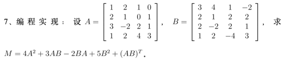
| import numpy as np
A = np.array([[1, 2, 1, 0],
[2, 1, 0, 1],
[3, -2, 2, 1],
[1, 2, 4, 3]])
B = np.array([[3, 4, 1, -2],
[2, 1, 1, 2],
[2, -2, 2, 1],
[1, 2, -4, 3]])
M = 4 * np.dot(A, A) + 3 * np.dot(A, B) - 2 * np.dot(B, A) + 5 * np.dot(B, B) + np.dot(A, B).T
print(M)
|
[[129  71 128  26]
 [ 93 113 -10  32]
 [ 84  51  28 -25]
 [155  85 -19 141]]
8、编程解决如下金融公司支付基金的流动问题:金融机构为保证现金充分支付,设立—笔总额8600万元的基金,分开放置在位于甲城和乙城的两家公司,基金在平时可以使用,但每周末结算时必须确保总额仍然为8600万元。经过相当长的一段时期的现金流动,发现每过一周,各公司的支付基金在流通过程中多数还留在自己的公司内,而甲城公司有l5%支付基金流动到乙城公司,乙城公司则有l8%支付基金流动到甲城公司。起初甲城公司基金为4l00万元,乙城公司基金为4600万元。按此规律,两公司支付基金数额变化趋势如何?如果金融专家认为每个公司的支付基金不能少于3900万元,那么是否需要在必要时调动基金?
1
2
3
4
5
6
7
8
9
10
11
12
13
14
15
16
17
18
19
20
21
22
23
24
25
26
27
28
29
30
31
32
33
34
35
36
37
38
39
40
|
import numpy as np
A = np.array([[1, 2, 1, 0],
[2, 1, 0, 1],
[3, -2, 2, 1],
[1, 2, 4, 3]])
B = np.array([[3, 4, 1, -2],
[2, 1, 1, 2],
[2, -2, 2, 1],
[1, 2, -4, 3]])
M = 4 * np.dot(A, A) + 3 * np.dot(A, B) - 2 * np.dot(B, A) + 5 * np.dot(B, B) + np.dot(A, B).T
print(M)
transition_matrix = np.array([[0.85, 0.18],
[0.15, 0.82]])
funds_distribution = np.array([[4100],
[4500]])
for week in range(1, 53):
funds_distribution = np.dot(transition_matrix, funds_distribution)
if funds_distribution[0] < 3900 or funds_distribution[1] < 3900:
print(f"在第 {week} 周需要调动基金。")
break
print(f"一年后甲城公司基金为:{funds_distribution[0][0]}万元")
print(f"一年后乙城公司基金为:{funds_distribution[1][0]}万元")
|
[[129  71 128  26]
 [ 93 113 -10  32]
 [ 84  51  28 -25]
 [155  85 -19 141]]
一年后甲城公司基金为:4690.909090375244万元
一年后乙城公司基金为:3909.090909624741万元
9、编程计算全0、全1、单位二阶方阵的特征值与特征向量,并给出相应结果。
1
2
3
4
5
6
7
8
9
10
11
12
13
14
15
16
17
18
19
20
21
22
23
24
25
26
| import numpy as np
from numpy.linalg import eig
A1 = np.zeros((2,2))
A2 = np.ones((2,2))
A3 = np.eye(2)
eig_vals1, eig_vecs1 = eig(A1)
eig_vals2, eig_vecs2 = eig(A2)
eig_vals3, eig_vecs3 = eig(A3)
print("全0矩阵的特征值和特征向量:")
print("特征值:", eig_vals1)
print("特征向量:\n", eig_vecs1)
print("\n全1矩阵的特征值和特征向量:")
print("特征值:", eig_vals2)
print("特征向量:\n", eig_vecs2)
print("\n单位矩阵的特征值和特征向量:")
print("特征值:", eig_vals3)
print("特征向量:\n", eig_vecs3)
|
全0矩阵的特征值和特征向量:
特征值: [0. 0.]
特征向量:
 [[1. 0.]
 [0. 1.]]

全1矩阵的特征值和特征向量:
特征值: [2. 0.]
特征向量:
 [[ 0.70710678 -0.70710678]
 [ 0.70710678  0.70710678]]

单位矩阵的特征值和特征向量:
特征值: [1. 1.]
特征向量:
 [[1. 0.]
 [0. 1.]]
10、编程求向量的曼哈顿距离、欧氏距离和切比雪夫距离。
1
2
3
4
5
6
7
8
9
10
11
12
13
14
15
16
| from scipy.spatial import distance
vector_a = np.array([1, 2, 3])
vector_b = np.array([4, 5, 6])
manhattan_dist = distance.cityblock(vector_a, vector_b)
euclidean_dist = distance.euclidean(vector_a, vector_b)
chebyshev_dist = distance.chebyshev(vector_a, vector_b)
manhattan_dist, euclidean_dist, chebyshev_dist
|
(9, 5.196152422706632, 3)
11、用Python编程实现贝叶斯公式的计算:假设有两个教室各有l00个学生,A教室中有60个男生、40个女生,B教室中有30个男生、70个女生。假设随机选择其中一个教室,从里面叫出一个人记下性别再回到原来的教室,那么被选择的教室是A教室的概率有多大?
1
2
3
4
5
6
7
8
9
10
11
12
|
prob_A = 1/2
prob_B = 1/2
prob_boy_given_A = 60/100
prob_boy_given_B = 30/100
prob_A_given_boy = (prob_boy_given_A * prob_A) / (prob_boy_given_A * prob_A + prob_boy_given_B * prob_B)
prob_A_given_boy
|
0.6666666666666667
12使用批量梯度下降算法拟合直线。待拟合的二维平面数据点:(6, 7), (8, 9), (10, 13),(14, 17.5), (18, 18)。
1
2
3
4
5
6
7
8
9
10
11
12
13
14
15
16
17
18
19
|
def linear_regression(X, y, learning_rate=0.001, n_iterations=10000):
m = len(X)
X_b = np.c_[np.ones((m, 1)), X]
theta = np.random.randn(2, 1)
for iteration in range(n_iterations):
gradients = 2/m * X_b.T.dot(X_b.dot(theta) - y)
theta -= learning_rate * gradients
return theta
X = np.array([6, 8, 10, 14, 18]).reshape(-1, 1)
y = np.array([7, 9, 13, 17.5, 18]).reshape(-1, 1)
theta = linear_regression(X, y)
print(theta)
|
[[1.7207352 ]
 [0.99534866]]